Anomaly detection in IoT
Through the Internet of Things (IoT) we can collect data from the physical world through sensors. Examples include smart home devices, urban projects and even personal devices. One of the critical challenges in this connected ecosystem is anomaly detection: identifying when a device or sensor behaves unexpectedly, which can indicate malfunctions, environmental changes, or security breaches. Efficiently managing these anomalies is paramount to maintaining the reliability, efficiency, and security of IoT systems. In this blog we will explore two approaches to detect anomalies: batch processing with the Python data stack, and stream processing with Python and Bytewax.
Introducing the problem: air quality data
Air quality monitoring uses sensors distributed across various locations to collect data on pollutants like PM2.5, CO2 levels, and other harmful substances. This scenario is a classic IoT application where continuous data streams are generated. Anomalies in air quality data might include sudden spikes in pollutant levels or unexpected drops, which could indicate environmental hazards, equipment failures, or data integrity issues. Monitoring these anomalies is crucial for public health and environmental protection.
Processing data prior to detection
Before anomalies can be accurately detected, the data must be clean and complete. This involves processes such as imputation (filling in missing data), data cleanup (removing or correcting data anomalies that are not of analytical interest, like sensor malfunctions), and normalization. These steps are essential to ensure that the anomaly detection algorithms are working with high-quality data and that the insights derived from the data are accurate and reliable.
Let's take a look at two approaches: batch processing and stream processing.
Assumption
For both strategies, we will read from a file with data extracted from the Purple AIR API. To make a connection to the data directly, please review their documentation.
Strategy 1: batch processing
This strategy is implemented in full in this Jupyter notebook. It implements the JSON and pandas libraries for data wrangling, Scikit-learn for data imputation and River for anomaly detection.
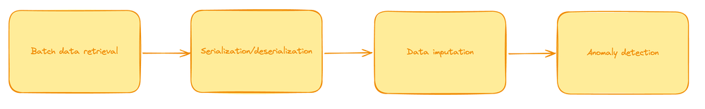
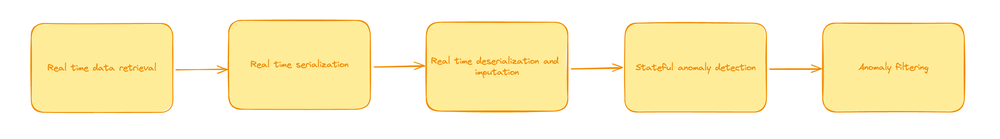
Batch Processing Steps
- Data Retrieval: Data is collected in large batches from storage or a database.
- Data Serialization/Deserialization: Data is formatted or parsed to be usable in processing tools.
- Data Imputation: Missing data points are filled using statistical methods.
- Anomaly Detection: Algorithms analyze the batch of data to identify outliers.
Let's take a look at the key areas in code responsible for each.
Data processing: serialization and deserialization
In this function, we take JSON response as input, and return a Python dictionary. These functions are in charge of flattening and wrangling the data for imputation.
def serialize(data):
    """
    This function serializes the data by converting it
    to a JSON string and then encoding it to bytes.

    Args:
    data: A dictionary containing the data to be serialized.

    Returns:
    A list of serialized data in bytes format.
    """
    headers = data['fields']
    serialized_data = []

    for entry in data['data']:
        try:
            # Create a dictionary for each entry, matching fields with values
            entry_data = {headers[i]: entry[i] for i in range(len(headers))}
            # Convert the dictionary to a JSON string and then encode it to bytes
            entry_bytes = json.dumps(entry_data).encode('utf-8')
            serialized_data.append(entry_bytes)
        except IndexError:
            # This block catches cases where the entry might not have all the fields
            print("IndexError with entry:", entry)
            continue

    return serialized_data


def deserialize(byte_objects_list):
    """
    This function deserializes the data by decoding the bytes
    it converts epoch time to a datetime object and converts
    "pm2.5_cf_1" to a float.

    Args:
    byte_objects_list: A list of byte objects to be deserialized.

    Returns:
    A list of dictionaries containing the deserialized data.
    """
    results = []  # List to hold the processed sensor data
    for byte_object in byte_objects_list:
        if byte_object:  # Check if byte_object is not empty
            sensor_data = json.loads(byte_object.decode('utf-8'))  # Decode and load JSON from bytes

            # Convert "pm2.5_cf_1" to a float, check if the value exists and is not None
            if 'pm2.5_cf_1' in sensor_data and sensor_data['pm2.5_cf_1'] is not None:
                sensor_data['pm2.5_cf_1'] = float(sensor_data['pm2.5_cf_1'])

            # Convert "date_created" from Unix epoch time to a datetime object, check if the value exists
            if 'date_created' in sensor_data and sensor_data['date_created'] is not None:
                sensor_data['date_created'] = datetime.fromtimestamp(sensor_data['date_created'], tz=timezone.utc)

            results.append(sensor_data)  # Add the processed data to the results list

    return results
Once the records have been processed, we can then impute missing values. For this step, we can use different methods. We chose Scikit-learn's KNN imputer. This function will use pandas and numpy array to iterate over the records and perform imputation. The resulting data is then converted to dictionary again.
def impute_data_with_knn(deserialized_data):
    """
    Takes a list of dictionaries from deserialized data, converts it into a DataFrame,
    performs KNN imputation, and converts it back into a list of dictionaries.

    Args:
    deserialized_data: A list of dictionaries containing sensor data.

    Returns:
    A list of dictionaries with imputed data.
    """
    # Convert list of dictionaries to DataFrame
    df = pd.DataFrame(deserialized_data)

    # Ensure all numeric columns are in appropriate data types
    for column in df.columns:
        if df[column].dtype == 'object':
            try:
                df[column] = pd.to_numeric(df[column])
            except ValueError:
                continue  # Keep non-convertible columns as object if needed

    # Apply KNN imputer to numeric columns
    numeric_columns = df.select_dtypes(include=[np.number]).columns
    imputer = KNNImputer(n_neighbors=5, weights='uniform')
    imputed_array = imputer.fit_transform(df[numeric_columns])

    # Update numeric columns in DataFrame with imputed values
    df[numeric_columns] = imputed_array

    # Convert DataFrame back to a list of dictionaries
    imputed_data = df.to_dict(orient='records')

    return imputed_data
Next, we will define an anomaly detector class using scikit-learn.
The Isolation Forest is a good choice for batch anomaly detection due to its effectiveness with multidimensional data and its capability of identifying anomalies without needing a target label. Here's how:
- Initialize the Isolation Forest: The detector is initialized with parameters such as the number of trees (n_estimators), the sample size (max_samples), and the contamination factor which represents the proportion of outliers expected in the data.
- Fit the Model: Since we are assuming batch processing, the model can be fitted on a predefined dataset. This dataset should ideally represent typical "normal" data to help the model learn the structure of non-anomalous data.
- Predict and Score Anomalies: After the model is fitted, it can predict new data points as anomalies based on the isolation properties learned during training. The
score_samplesfunction gives a raw anomaly score, which can be used to determine how anomalous a data point is.
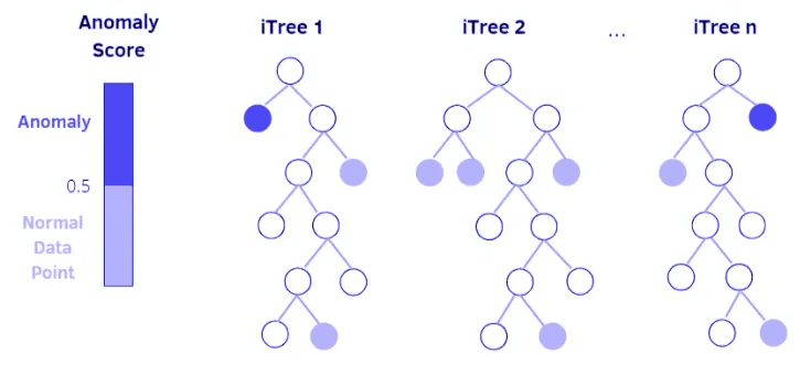
Image from Medium Article "Anomaly detection using Isolation Forest and Local Outlier Factor"
class AnomalyDetector:
    """
    Anomaly detector using Isolation Forest from scikit-learn
    """

    def __init__(self, n_estimators=100, max_samples='auto', contamination=0.01, random_state=42):
        """
        Initialize the anomaly detector with parameters suitable for Isolation Forest
        """
        self.detector = IsolationForest(
            n_estimators=n_estimators,
            max_samples=max_samples,
            contamination=contamination,
            random_state=random_state
        )

    def fit(self, data):
        """
        Fit the Isolation Forest model with data
        """
        self.detector.fit(data)

    def predict(self, data):
        """
        Predict data using the fitted model and tag entries as anomalies
        """
        # -1 for anomalies, 1 for normal
        predictions = self.detector.predict(data)
        scores = self.detector.score_samples(data)
        return predictions, scores
We can then execute all steps together as follows:
if __name__=="__main__":
    # Opening JSON file
    f = open('data.json')

    # returns JSON object as
    # a dictionary
    data = json.load(f)

    # Begin data processing
    # Serialize the data to bytes
    serialized_entries = serialize(data)
    # Deserialize the data and transform epoch
    deserialized_data = deserialize(serialized_entries)

    # Perform KNN imputation on deserialized data
    imputed_data = impute_data_with_knn(deserialized_data)

    # Prepare your data (assuming imputed_data is a DataFrame ready for input)
    detector = AnomalyDetector()

    # You must convert the list of dictionaries to a DataFrame if not already done
    df = pd.DataFrame(imputed_data)

    # Select only the numeric columns for anomaly detection
    numeric_columns = df.select_dtypes(include=[np.number])

    # Fit the model with numeric data
    detector.fit(numeric_columns)

    # Predict anomalies on the same or new data
    predictions, scores = detector.predict(numeric_columns)

    # Add predictions and scores back to the DataFrame for review or further processing
    df['anomaly'] = predictions
    df['score'] = scores

    # Print or process anomalies
    anomalies = df[df['anomaly'] == -1]

>>
sensor_index    date_created    rssi    uptime  latitude    longitude   humidity    temperature pressure    pm1.0   pm2.5_alt   pm10.0  pm1.0_cf_1  pm2.5_atm   pm2.5_cf_1  pm10.0_cf_1 anomaly score
100 1970.0  2017-07-11 18:58:30+00:00   -76.0   17419.0 33.998270   -118.437546 34.0    86.0    1013.58 2759.8  0.0 2759.8  4139.3  2759.8  4139.3  4139.3  -1  -0.743272
127 2334.0  2017-07-31 18:03:42+00:00   -55.0   231.0   41.045155   -111.985910 70.0    39.0    862.87  108.9   53.6    133.7   159.0   132.4   185.8   186.5   -1  -0.737338
Strengths
- Handles large datasets efficiently.
- Easier to manage and debug because of its sequential nature.
- Suitable for less time-sensitive applications.
Limitations
- Delays in processing can lead to outdated results.
- Less efficient in using computational resources due to sporadic processing loads.
- Struggles with real-time data ingestion and immediate anomaly detection.
Let's turn our attention to stream processing next.
Strategy 2: stream processing
This strategy is implemented in full in this Jupyter notebook. It implements the Bytewax library as the stream processing engine, JSON for data wrangling,and River for value imputation and anomaly detection.
Stream Processing Steps
- Data Ingestion: Data is continuously ingested in real-time.
- Data Serialization/Deserialization: Data is processed as it streams.
- Data Imputation: Missing values are immediately imputed.
- Anomaly Detection: Anomalies are detected on-the-fly.
To convert the serialize function into a Bytewax stream-equivalent format, we need to create a data source that behaves as a generator or a source of streaming data. Below, I will define two classes to model this behavior: one for partition-specific streaming data (SerializedData), and another to encapsulate the dynamic data generation across potentially multiple workers (SerializedInput).
Step 1: Define SerializedData as a StatelessSourcePartition This class will act as a source partition that iterates over a dataset, serializing each entry according to the provided headers and fields.
Step 2: Define SerializedInput as a DynamicSource This class encapsulates the partition management for the data source, ensuring that each worker in a distributed environment gets a proper instance of the source partition.
class SerializedData(StatelessSourcePartition):
    """
    Emit serialized data directly for simplicity. This class will serialize
    each entry in the 'data' list by mapping it to the corresponding 'fields'.
    """
    def __init__(self, full_data):
        self.fields = full_data['fields']
        self.data_entries = full_data['data']
        self.metadata = {k: v for k, v in full_data.items() if k not in ['fields', 'data']}
        self._it = iter(self.data_entries)

    def next_batch(self):
        try:
            data_entry = next(self._it)
            # Map each entry in 'data' with the corresponding field in 'fields'
            data_dict = dict(zip(self.fields, data_entry))
            # Merge metadata with data_dict to form the complete record
            complete_record = {**self.metadata, **{"data": data_dict}}
            # Serialize the complete record
            serialized = json.dumps(complete_record).encode('utf-8')
            return [serialized]
        except StopIteration:
            raise StopIteration


class SerializedInput(DynamicSource):
    """
    Dynamic data source that partitions the input data among workers.
    """
    def __init__(self, data):
        self.data = data
        self.total_entries = len(data['data'])

    def build(self, step_id, worker_index, worker_count):
        # Calculate the slice of data each worker should handle
        part_size = self.total_entries // worker_count
        start = part_size * worker_index
        end = start + part_size if worker_index != worker_count - 1 else self.total_entries

        # Create a partition of the data for the specific worker
        # Note: This partitions only the 'data' array. Metadata and fields are assumed
        # to be common and small enough to be replicated across workers.
        data_partition = {
            "api_version": self.data['api_version'],
            "time_stamp": self.data['time_stamp'],
            "data_time_stamp": self.data['data_time_stamp'],
            "max_age": self.data['max_age'],
            "firmware_default_version": self.data['firmware_default_version'],
            "fields": self.data['fields'],
            "data": self.data['data'][start:end]
        }

        return SerializedData(data_partition)
The SerializedData class now takes the entire data structure, keeps the metadata, and iterates over the data list. Each entry in data is mapped to the corresponding field specified in fields, combined with the metadata, serialized into a JSON string, and then encoded.
Integration into Dataflow: The class is used directly within a Bytewax dataflow as an input source, demonstrating how serialized data would be produced from the structured input.
We can then deserialize the data with a simple function.
In this function, we will also perform imputation of missing values, particularly, for the temperature, humidity, pressure attributes and PM attributes.
Unlike the batch version, we will use the river library to perform imputation, this is due to the library's compatibility with stream processing.
temp_imputer = preprocessing.StatImputer(("temperature", stats.Mean()))
humidity_imputer = preprocessing.StatImputer(("humidity", stats.Mean()))
pressure_imputer = preprocessing.StatImputer(("pressure", stats.Mean()))
pm1_imputer = preprocessing.StatImputer(("pm1.0_cf_1", stats.Mean()))


def process_and_impute_data(byte_data):
    """Deserialize byte data, impute missing values, and prepare for stateful processing."""
    # Deserialize the byte data
    record = json.loads(byte_data.decode('utf-8'))
    sensor_data = record['data']
    key = str(sensor_data.get("sensor_index", "default"))

    # Impute missing values
    for item in [temp_imputer, humidity_imputer, pressure_imputer, pm1_imputer]:
      item.learn_one(sensor_data)
      sensor_data = item.transform_one(sensor_data)
    temp_imputer.learn_one(sensor_data)  # Update imputer with current data
    sensor_data = temp_imputer.transform_one(sensor_data)  # Impute missing values

    # Return the processed data with the key
    return (key, sensor_data)
Unlike the batch example, we will use the river library's HalfSpaceTrees for detecting anomalies in streaming data.
River is specifically designed for online learning, which is a type of incremental learning where the model updates continuously as each data point arrives. This is crucial for applications that receive data continuously and require real-time learning and predictions. In contrast, scikit-learn primarily supports batch learning where the model sees all the training data at once and learns from this complete set. River allows for models to adapt quickly to changes in the data distribution (concept drift) without needing to retrain from scratch.
Using River facilitates the easy adaptation of models to new data patterns and anomalies, which is particularly valuable in dynamic environments such as financial markets, IoT device monitoring, or real-time threat detection systems.
This class is integral for real-time anomaly detection. It maintains a model state across the data stream, continuously learning and scoring new data points.
class StatefulAnomalyDetector:
    """
    This class is a stateful object that encapsulates an anomaly detection model
    from the River library and provides a method that uses this model to detect
    anomalies in streaming data. The detect_anomaly method of this object is
    passed to op.stateful_map, so the state is maintained across calls to this
    method.
    """
    def __init__(self, n_trees=10, height=8, window_size=72, seed=11, limit=(0.0, 1200)):
        self.detector = anomaly.HalfSpaceTrees(
            n_trees=n_trees,
            height=height,
            window_size=window_size,
            limits={'pm1.0_cf_1': limit},  # Ensure these limits make sense for your data
            seed=seed
        )

    def detect_anomaly(self, key, data):
        """
        Detect anomalies in sensor data and update the anomaly score in the data.
        """
        value = data.get('pm1.0_cf_1')
        if value is not None:
            try:
                value = float(value)
                score = self.detector.score_one({'pm1.0_cf_1': value})
                self.detector.learn_one({'pm1.0_cf_1': value})
                data['anomaly_score'] = score
            except ValueError:
                print(f"Skipping entry, invalid data for pm1.0_cf_1: {data['pm1.0_cf_1']}")
                data['anomaly_score'] = None
        else:
            data['anomaly_score'] = None
        return key, data
To ensure we only call the anomalies, we can set up a filtering function.
def filter_high_anomaly(data_tuple):
    """Filter entries with high anomaly scores."""
    key, data = data_tuple
    # Check if 'anomaly_score' is greater than 0.7
    return data.get('anomaly_score', 0) > 0.7
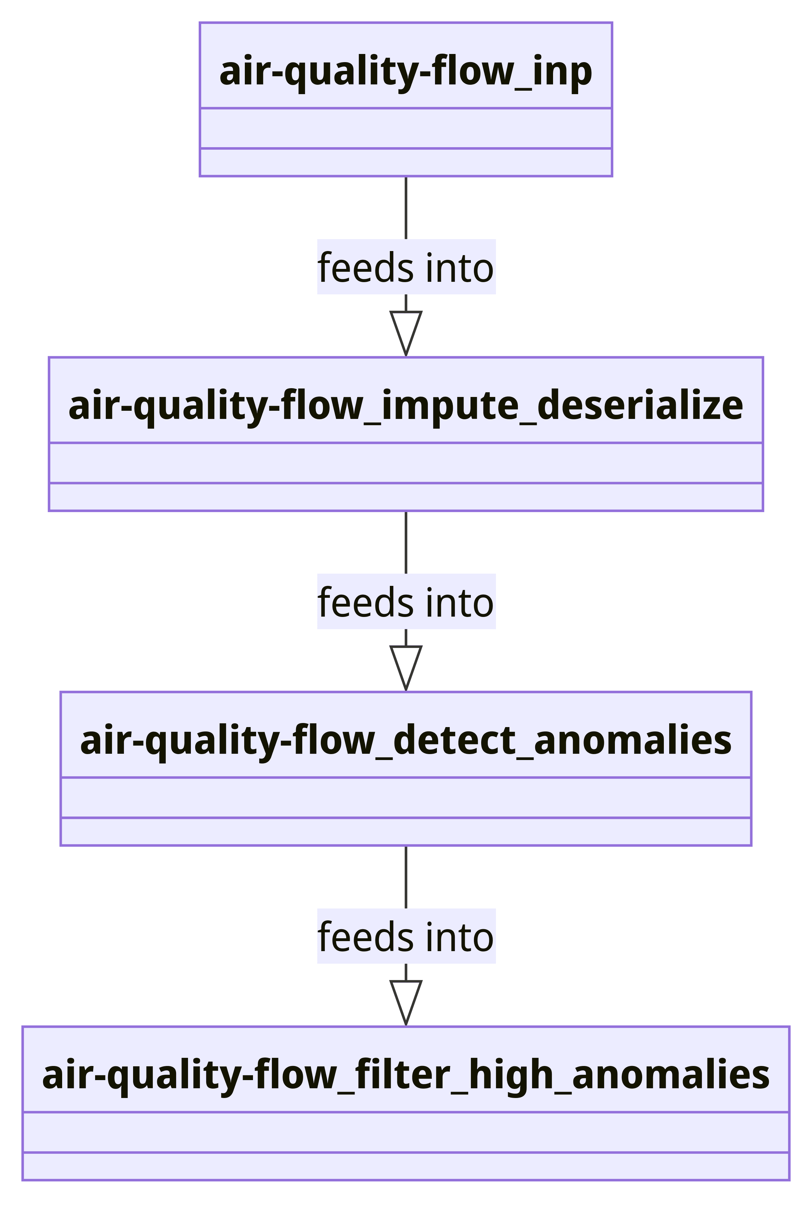
Bringing all pieces together into a dataflow, we can define
# Setup the dataflow
flow = Dataflow("air-quality-flow")
inp = op.input("inp", flow, SerializedInput(data))
impute_deserialize = op.map("impute_deserialize", inp, process_and_impute_data)


# Add anomaly detection to the dataflow
anomaly_detector = StatefulAnomalyDetector()
detect_anomalies_step = op.stateful_map("detect_anomalies", impute_deserialize, anomaly_detector.detect_anomaly)

# Detect anomalies within threshold
filter_anomalies = op.filter("filter_high_anomalies", detect_anomalies_step, filter_high_anomaly)


# Output or further processing
op.inspect("inspect_filtered_anomalies", filter_anomalies)


run_main(flow)

>>
air-quality-flow.inspect_filtered_anomalies: ('1479', {'sensor_index': 1479, 'date_created': 1492800687, 'rssi': -56, 'uptime': 31089, 'latitude': 36.005188, 'longitude': -78.85404, 'humidity': 56, 'temperature': 77, 'pressure': 1001.59, 'pm1.0': 21.4, 'pm2.5_alt': 15.6, 'pm10.0': 30.2, 'pm1.0_cf_1': 22.8, 'pm2.5_atm': 28.3, 'pm2.5_cf_1': 28.5, 'pm10.0_cf_1': 30.2, 'anomaly_score': 0.8223961730811046})
air-quality-flow.inspect_filtered_anomalies: ('1525', {'sensor_index': 1525, 'date_created': 1493500594, 'rssi': -69, 'uptime': 10390, 'latitude': 22.528564, 'longitude': 113.94328, 'humidity': 64, 'temperature': 88, 'pressure': 1012.97, 'pm1.0': 23.5, 'pm2.5_alt': 20.8, 'pm10.0': 39.1, 'pm1.0_cf_1': 26.5, 'pm2.5_atm': 33.8, 'pm2.5_cf_1': 36.7, 'pm10.0_cf_1': 39.2, 'anomaly_score': 0.8352685366383996})
This flow can be represented as a mermaid graph as follows:
The complete dataflow file can be found here
And executed from a terminal as follows.
python -m bytewax.run dataflow:flow
Strengths
- Real-time data processing allows for immediate detection and response.
- More efficient in resource utilization as data is processed incrementally.
- Adapts quickly to changes in data patterns.
Limitations
- Requires more complex system architecture.
- Potentially higher overheads for managing continuous data flows.
- Ensuring data consistency and managing state across distributed systems can be challenging.
Batch processing or Stream processing?
The real-time processing flow described using Bytewax and the discrete example outlined in the batch processing notebook represent two fundamentally different approaches to handling and analyzing data, especially concerning how data is ingested, processed, and utilized for anomaly detection. Here's a detailed comparison:
| Aspect | Real-Time Stream Processing | Batch Processing |
|---|---|---|
| Data Ingestion and Handling | ||
| Continuous Input | Data is continuously ingested as it is generated. The SerializedInput class handles data as a stream, breaking it down into partitions that are processed independently by different workers. Scalable and efficient. | Data is typically loaded in large chunks at scheduled intervals. Delays occur as the system must wait for a complete batch of data before beginning processing. |
| Incremental Processing | Each piece of data is processed incrementally as it arrives, effective for applications where data is generated continuously, such as environmental monitoring. | The entire dataset or substantial chunks of it are processed at once. This can be resource-intensive and less efficient if the data size is significant or if only a small portion of the data needs updating or re-evaluation. |
| Processing Steps and Dataflow | ||
| Dynamic Data Flow | Dataflow is explicitly defined as a sequence of operations (op.map, op.filter, etc.) that data passes through. Each function in the flow is designed to handle data as it streams through the system. | Each step (deserialization, imputation, anomaly detection) is generally performed once per batch. The entire dataset must often be loaded into memory, processed, and then outputted, leading to inefficiencies. |
| Stateful and Stateless Operations | Some operations like anomaly detection are stateful and maintain information across different data points. Others, like deserialization, are stateless and operate independently on each data point. | All steps are repeated from scratch each time a new batch is processed, even if only minor changes exist between batches. This can result in redundant processing and increased computational load. |
| Adaptability to Changes | ||
| High Responsiveness | By continuously processing data as it arrives, the system can quickly adapt to changes in data characteristics or detect anomalies in real time, crucial for environments where conditions change rapidly. | Changes in data patterns or new anomalies might only be detected once a new batch is processed, leading to delays in responding to critical events or shifts in data trends. |
| Continuous Learning | The model parameters can be updated incrementally, allowing the anomaly detection models to adapt to new trends or changes in the data without requiring a complete retraining. | Model updates or retraining usually happen at fixed intervals, depending on the batch schedule, which might not be sufficient for rapidly changing data sources. |
While both methods have their applications, the choice between real-time stream processing and batch processing depends largely on the nature of the data and the requirements of the application. Real-time processing is better suited for scenarios where timely data analysis is crucial and data is continuously generated, while batch processing might be preferred when data volumes are large, and less frequent processing is acceptable.
Future blogs
In this blog, we explored two approaches to clean and detect anomalies from IoT data. In a future blog, we will explore how to deploy a stream-processing solution.
Streaming Data for Data Scientists: Part 1

Laura Funderburk
Senior Developer AdvocateLaura Funderburk holds a B.Sc. in Mathematics from Simon Fraser University and has extensive work experience as a data scientist. She is passionate about leveraging open source for MLOps and DataOps and is dedicated to outreach and education.